D3 and Livescript is like Peanut Butter and Chocolate

Livescript is an awesome... somewhat new language that doubles down on functional programming. It directly compiles into Javascript, much like Typescript and Coffeescript.

I spend a lot of time with D3 and Javascript. D3, in short, is a data visualization library for Javascript that is very declarative in nature.

If you're familiar with D3 you spend a lot of time doing things like this:

d3.selectAll(".bars")
    .style("fill", function (data) {
        return data.colour;
    });

This is a silly example that selects all elements having class bar. Then changes their colour to whatever is stored in the colour property bound to that element.

With Livescript it looks like this:

d3.selectAll ".bars"
    .style "fill", (data) -> data.colour

This works too:

d3.selectAll '.bars'
    .style 'fill', -> it.colour

Or even this

d3.selectAll \.bars
    .style \fill, (.colour)

Once you get used to the lack of parentheses it starts to makes sense on one line.

d3.selectAll \.bars .style \fill, (.colour)

I highly recommend having a look. https://livescript.net/

Morphing Between SVG Shapes

In order to animate between two shapes in SVG you need an equal number of nodes. This is because the node coordinates are what get adjusted during a transition. If one shape has more then another you get some really weird behaviour.

One approach is to manually edit one of the paths so the number of nodes matches the other. But that is pretty time consuming. I opt for the lazy approach of stuffing it through a filter.

I wrote polymorph to make the calculation between two shapes. Essentially transposing the nodes from one shape onto the path of another.

Input Shape

This is a little over simplified... But you start with a complex shape with lots of nodes.

Destination Shape

Then say you want to animate it into a simple circle like this.

Note the destination path contains arcs. Polymorph can handle any type of SVG path for the destination. The source, and more complex, path must always contain linear lines. See SVG Path for more details.

var inputShape = "m 14.108932,44.306697 33.663417,-22.772311 49.257499,-6.435654 4.702982,24.504988 -13.613886,30.693115 42.326796,10.14853 44.80204,-10.14853 8.91091,30.940645 -3.46535,31.18816 -28.46539,23.51489 L 99.752625,177.72274 87.128843,144.55437 97.277373,118.56423 75.000112,97.029549 30.44559,94.059247 44.059472,65.841383 14.108932,44.306697"

var destinationShape = "m 191.90169,310.3161 a 51.514591,51.514591 0 1 1 -103.029181,0 51.514591,51.514591 0 1 1 103.029181,0 z"

var newShape = polymorph.transpose(inputShape,destinationShape);

New Shape

The nodes are obviously enlarged for the purposes of this post. But you end up with a shape that is almost identical to the Destination Shape. However, the node numbers match.

You can transpose nodes in any direction. However it makes most sense to convert from high to equal or less complexity.







Now use one of the handy dandy svg libraries, such as snap, velocity, or d3, to transform between the two. The following example uses d3 to transform from geographic boundaries (just svg paths) into circles, and back again.

See the Pen Morphing land shapes to random circles by Jamie Popkin (@jamiepopkin) on CodePen.

Animating a geographic boundary into a circle.. Then back again.

Paths in SVG are comprised of points called nodes. In order to transition from one path (the boundary) into another (the circle) the same number of nodes need to exist on both.

Start by drawing a boundary (Texas) with D3.

See the Pen Texas Boundary With D3 by Jamie Popkin (@jamiepopkin) on CodePen.

We want to shrink into a circle that is centred around the centroid of Texas. D3 has a method for finding the centroid. We use this to draw paths from the centroid to each node.

See the Pen Texas With Spokes by Jamie Popkin (@jamiepopkin) on CodePen.

SVG has a handy dandy method for placing a node along the specified distance of a path, getPointAtLength. We use this to calculate a new point at whatever distance from the centroid. In this example we use a radius of 10 pixels. The nice thing about this approach is we can be assured all nodes in the original boundary are accounted for and have a place in the circle.

See the Pen Texas With Spokes and Inner Circle Nodes by Jamie Popkin (@jamiepopkin) on CodePen.

Finally create a path from the new nodes. We use this to animate the original polygon. D3 makes this pretty simple with the transition method.

Voilà.

See the Pen Shrinking Texas With D3 by Jamie Popkin (@jamiepopkin) on CodePen.

Upgrading to PostGIS 2.0 on Ubuntu

Like most projects... I felt it paramount to utilize the latest bleeding edge technology to get the job done. Or at least that's how I rationalize playing with something new. Recently I needed to run an analysis on both vector and raster data in PostGIS. This meant upgrading to PostGIS 2.0. Which happened to be absent from the standard Ubuntu repository.

No worries... This is how I got it installed and running in a pre-existing database.:

First upgrade to the latest version of Ubuntu. At the moment it's 12.10 (quantal). You can find your current version by typing lsb_release  -a at the command line.

Backup whatever database you want to upgrade:

pg_dump -Fc -b -v -f fb_19jan2012.backup fb

Purge the old install of postgis

sudo aptitude purge postgis

Install the Ubuntu gis repo from the Ubuntu GIS group and update. At the moment you have to install the unstable version in order for it to work with quantal.

sudo apt-add-repository ppa:ubuntugis/ubuntugis-unstable
sudo aptitude update

Install the new postgis. It should automatically choose the new version. It actually conflicts with the older version... But doesn't seem to complain about it.

sudo aptitude install postgis

Setup a new database. I'm calling it fb2.

sudo su postgres
createdb fb2
psql -d fb2 -f /usr/share/postgresql/9.1/contrib/postgis-2.0/postgis.sql
psql -d fb2 -f /usr/share/postgresql/9.1/contrib/postgis-2.0/spatial_ref_sys.sql
psql -d fb2 -f /usr/share/postgresql/9.1/contrib/postgis-2.0/rtpostgis.sql
psql -d fb2 -f /usr/share/postgresql/9.1/contrib/postgis_comments.sql
psql -d fb2 -c "grant all privileges on database fb2 to some_user"

Now we can stuff the backup into our new database with the handy perl command, postgis_restore.pl, that came with the install. Make sure you get out of the postgres account first.

exit
/usr/share/postgresql/9.1/contrib/postgis-2.0/postgis_restore.pl fb_19jan2012.backup | psql fb2

Happy day! PostGIS 2.0 is installed on our database.

Then I was able to load a digital elevation model raster like this.

raster2pgsql -s 4326 -I -M -C -t 25x25 dem_wa.tif dem_wa > dem_wa.sql
psql fb2 < dem_wa.sql

TADA!

The first raster layer in the new PostGIS 2.0 database. Displayed with qGIS.

Resources:

• Ubuntu GIS group
• Linfiniti Geo Blog

Creating a Terrain Wetness Index from a Digital Elevation Model

A Terrain Wetness Index (TWI) is a means for measuring drainage in a landscape. In particular, areas with poor drainage. The purpose is to isolate dips and hollows that maintain water for longer periods, exclusive of permanent water bodies like lakes and swamps.

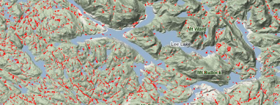
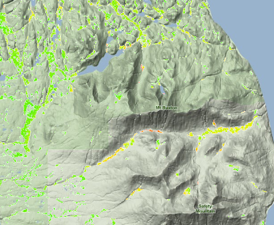
Areas identified as high value within the Terrain Wetness Index.
Located in Mainland British Columbia, East of the Northern tip of Vancouver Island.

A Digital Elevation Model (DEM) was acquired at 25 meter resolution. It was in an older ESRI grid format and separated into tiles.

I'm too cheap to buy ArcInfo... So I use Grass. First job is to import the grids:

r.in.gdal input=tdem092k.asc output=tdem092k
r.in.gdal input=tdem092l.asc output=tdem092l
...

Next is to merge them together:

 r.series input=tdem092k, tdem092l, tdem092m, tdem092n, tdem093c, tdem093d, tdem093e, tdem093f, tdem102i, tdem102p, tdem103a, tdem103h output=dem method=average

Now we have a seamless dataset to work with called dem. Time to do the real work.

Elevation Variance

Areas of high negative elevation variance.

The simplest way to calculate TWI is to run an elevation variance algorithm on the DEM. Simply put... This is a neighbor function that looks at the average elevation of all surrounding cells. Then calculates variance based on itself and the average.

To do this, two separate commands were required. The first calculated mean elevation for each cell:

r.neighbors -c input=dem output=mean3 size=3

This produced a dataset (mean3) holding the mean elevation for a window of 3x3. Considering the cells are 25 meters.. This resulted in a 75 by 75 meter window. The r.neighbors command defaults to mean as the function so it isn't necessary to specify it on the command line.

The second step is to calculate variance by comparing each elevation value in the original dem with the new mean values. Grass's extremely powerful and versitile r.mapcalc command is used for this.

r.mapcalc mean3diff = dem - mean3

We are looking for the dips only. Not the peaks. Peaks have positive values whereas dips have negative values. So we need to select for the negative variance values:

 r.mapcalc mean3dip = "if(mean3diff < 0, mean3diff, 0)"

These steps were repeated for different sized windows; 7 and 15. Then the three were added up:

r.series input=mean3dip,mean7dip,mean15dip output=dips method=sum

The result is illustrated above.

You may have noticed the image clearly identifies steep river valleys. This isn't exactly what we are after. We want to find low lying areas of poor drainage. We got low lying areas of high drainage.

Calculating mean elevation variance alone results in something like the following:

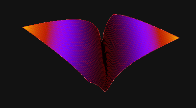
Terrain shape isolated by Mean Elevation Variance.

We are after a closed shape. Kinda like this:

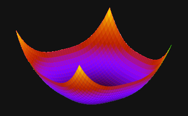
A closed dip resulting from the combination of Mean Elevation Variance
and  Mean Aspect Variance.

To achieve this we need to add another variable... Aspect variance.

Aspect Variance

Aspect is a term for terrain direction... Or the direction in which a slope is facing. If we apply the process above to aspect we can expect to isolate areas of high aspect variance.

Generate an aspect layer from the DEM with the r.slope.aspect command:

r.slope.aspect elevation=dem aspect=aspect

This creates a layer called aspect which contains continuous, floating point values of aspect in degrees. It is hard to correctly measure variance with continuous data. So, the next step is cluster the values into four classes; North, South, East, and West (identified numerically as 1-4). Mapcalc takes care of that:

r.mapcalc aspect_rc = "if(aspect > 45 && aspect <= 135, 1) + if(aspect > 135 && aspect <= 225, 2) + if(aspect > 225 && aspect <= 315, 3) + if(aspect <= 45 && aspect > 0, 4) + if(aspect > 315 && aspect <= 360, 4) + if(aspect == 0,null())"

Now we can run the variance precedure:

r.neighbors -c input=aspect_rc output=variance3aspect size=3 \
method=variance
r.neighbors -c input=aspect_rc output=variance7aspect size=7 \
method=variance
r.neighbors -c input=aspect_rc output=variance15aspect size=15 \
method=variance
r.series input=variance3aspect,variance7aspect,variance15aspect \
output=aspects_3_15 method=sum

Creating the Final Terrain Wetness Index

After reviewing both datasets, aspects_3_15 and dips, it was determined to select areas based on the following:

• Aspect Variance greater and equal to 10
• Mean elevation Variance less then -10

Another mapcalc statement takes care of this:

r.mapcalc twi = "if(aspects_3_15 >= 10 && dips < -10, dips, null())

When the criteria are met the resulting cells are populated with elevation variance. This allows for a gradient of depth for dips and hollows. All cells not selected are populated with null values.

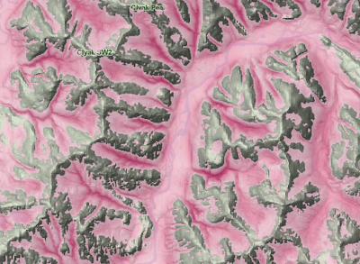
The result is our final Topographic Wetness Index and looks like this:

Final Topographic Wetness Index model

This has proven to be a valuable input to a model I am currently working on. If you want to see it in action take a look at the Yellow Cedar Decline Mashup.

Jamie

Calculating Togographic Exposure With Grass

Topographic exposure, also known as TOPEX, is a measure of surrounding landforms and how they effect wind. This post shows how to generate a TOPEX model based on a digital elevation model. The tool of choice was GRASS. The free and extremely powerful open source GIS system.

The goal of the analysis was to identify areas of low topographic exposure.
The red areas illustrate low exposure.

Exposure is calculated based on the height and distance of the surrounding horizon. These two measures combine to form the angle of inflection. It is this angle that we use to quantify topographic exposure. When a large topographic feature, like a mountain, is far in the distance the angle of inflection is low.

The angle of inflection is 45 degrees from the horizon

When the same mountain is closer the angle of inflection is higher. Therefore higher angle of inflection is equal to lower exposure or higher protection.

The angle of inflection is 75 degrees from the horizon

Based on advice from the windthrow expert Dr Stephen J Mitchell, it was determined to calculate the angle of inflection at 100 meter intervals from 100 to 2000 meters. The maximum angle was then extracted to define the true value of exposure. This of course needs to be calculated for each cell within the raster dataset. Within GRASS this is accomplished with the r.mapcalc command. 

First a little about neighbor calculations in GRASS. When we are looking at different spots in the horizon, we are essentially performing a neighbor function. The proper language for this is:

dem[3,1]

This translates into the raster cell three up and one to the right of the current cell. So if we wanted to subtract every cell in layer dem from the one that is three up and one to the right it would look like this.

r.mapcalc newlayer = dem[3,1] - dem

Not sure why you'd want to do that.... But there you go.

Now let's look at our topex equation. To calculate the angle of inflection we need to get the atan of height difference divided by the distance. This was determined based on simple trigonometry. The grass equation looks like this:

r.mapcalc incl4north = "atan(((dem - dem[4,0])) / ((25 * 4)))"

This creates a layer incl4north which holds the angle of inclination for 4 cells to the North. Note we now need brackets around the equation. The dem and all subsequent raster layers have 25 meter cells. This is used to calculate the distance by multiplying by the number of cells. This one calculation creates a raster layer containing the exposure for 100 meters in just one direction.

The goal is to take the maximum inclination for all distances from 100m to 2000m. Luckily there is a max() function for the r.mapcalc command. The following command calculates the maximum inclination for all intervals to the North:

r.mapcalc topex_n = "max(atan(((dem - dem[4,0])) / ((25 * 4))), \
atan(((dem[8,0] - dem)) / ((25 * 8))), \
atan(((dem[12,0] - dem)) / ((25 * 12))), \
atan(((dem[16,0] - dem)) / ((25 * 16))), \
atan(((dem[20,0] - dem)) / ((25 * 20))), \
atan(((dem[24,0] - dem)) / ((25 * 24))), \
atan(((dem[28,0] - dem)) / ((25 * 28))), \
atan(((dem[32,0] - dem)) / ((25 * 32))), \
atan(((dem[36,0] - dem)) / ((25 * 36))), \
atan(((dem[40,0] - dem)) / ((25 * 40))), \
atan(((dem[44,0] - dem)) / ((25 * 44))), \
atan(((dem[48,0] - dem)) / ((25 * 48))), \
atan(((dem[52,0] - dem)) / ((25 * 52))), \
atan(((dem[56,0] - dem)) / ((25 * 56))), \
atan(((dem[60,0] - dem)) / ((25 * 60))), \
atan(((dem[64,0] - dem)) / ((25 * 64))), \
atan(((dem[68,0] - dem)) / ((25 * 68))), \
atan(((dem[72,0] - dem)) / ((25 * 72))), \
atan(((dem[76,0] - dem)) / ((25 * 76))), \
atan(((dem[80,0] - dem) / ((25 * 80))))"

Now we need to do the same for the remaining 7 directions; NE, E, SE, S, SW, W, & NW. East, South and West are simple. Just rearrange the existing values. The remaining directions require a little more trigonometry. The hypotenuse is still the constant of 25 * (the number of cells). However the remaining side of the triangle requires the following equation:

cos(45) * (25 * # cells)

I chose to calculate this in perl with a function like this:

# Calculate one side of a right Isosceles triangle.
sub is () {
   $value = floor(cos(deg2rad(45)) * $_[0]);
   return $value;
}

Then plug the function into the mapcalc command like this:

atan(((dem - dem[" . is(4) . "," . is(4) . "])) / ((25 * 4)))

This is just the way I decided to do it. You could use that same trigonometry formula however you choose.

At this point we should have eight exposure raster layers. All that is required now is merge them together adding up the values. The command r.series does this beautifully:

 r.series input=topex_n,topex_ne,topex_e,topex_se,topex_s,topex_sw, \
topex_w,topex_nw output=topex method=sum

Viola!... We now have a complete TOPEX layer... Called topex.

TOPEX highlighting areas of low exposure.
Draped over Google's Terrain basemap.

To make use of the layer outside GRASS I like to convert it to a geotiff like this:

r.out.gdal -c input=topex createopt="COMPRESS=LZW" \
output=topex.tif nodata=0

If you have the GDAL library installed you can also generate a pyramid on it like this:

gdaladdo topex.tif 2 4 8 16 32 64

Now the dataset can be moved around and consumed by most GIS software; ArcGIS, Quantum, Geoserver, etc...

Jamie